Boids
To get started with agent-based modelling, we’ll recreate the classic Boids simulation of flocking behavior. This is a relatively simple example but it produces very pleasing visualizations.
Setup
We’re assuming you’ve read through the material in
getting started and are working in your
vivarium_examples package. If not, you should go there first.
Todo
package setup with __init__ and stuff
Building a population
Create a file called population.py with the following content:
~/code/vivarium_examples/boids/population.py 1# docs-start: imports
2import pandas as pd
3
4from vivarium.engine import Component
5from vivarium.engine.framework.engine import Builder
6from vivarium.engine.framework.population import SimulantData
7
8# docs-end: imports
9
10
11class Population(Component):
12 ##############
13 # Properties #
14 ##############
15
16 # docs-start: configuration_defaults
17 CONFIGURATION_DEFAULTS = {
18 "population": {
19 "colors": ["red", "blue"],
20 }
21 }
22 # docs-end: configuration_defaults
23
24 #####################
25 # Lifecycle methods #
26 #####################
27
28 # docs-start: setup
29 def setup(self, builder: Builder) -> None:
30 self.colors = builder.configuration.population.colors
31 self.randomness = builder.randomness.get_stream(self.name)
32 builder.population.register_initializer(
33 initializer=self.initialize_population,
34 columns=["color", "entrance_time"],
35 required_resources=[self.randomness],
36 )
37
38 # docs-end: setup
39
40 ########################
41 # Event-driven methods #
42 ########################
43
44 def initialize_population(self, pop_data: SimulantData) -> None:
45 new_population = pd.DataFrame(
46 {
47 "color": self.randomness.choice(pop_data.index, self.colors),
48 "entrance_time": pop_data.creation_time,
49 },
50 index=pop_data.index,
51 )
52 self.population_view.initialize(new_population)
Here we’re defining a component that generates a population of boids. Those boids are then randomly chosen to be either red or blue.
Let’s examine what’s going on in detail, as you’ll see many of the same patterns repeated in later components.
Imports
import pandas as pd

from vivarium.engine import Component
from vivarium.engine.framework.engine import Builder
from vivarium.engine.framework.population import SimulantData
NumPy is a library for doing high performance
numerical computing in Python. pandas is a set
of tools built on top of numpy that allow for fast
database-style querying and aggregating of data. Vivarium uses
pandas.DataFrame objects as it’s underlying representation of the
population and for many other data storage and manipulation tasks.
By convention, most people abbreviate these packages as np and pd
respectively, and we’ll follow that convention here.
Population class
Vivarium components are expressed as Python classes. You can find many resources on classes and object-oriented programming with a simple Google search. We’ll assume some fluency with this style of programming, but you should be able to follow along with most bits even if you’re unfamiliar.
Configuration defaults
In most simulations, we want to have an easily tunable set up knobs to adjust
various parameters. Vivarium accomplishes this by pulling those knobs out as
configuration information. Components typically expose the values they use in
the configuration_defaults class attribute.
CONFIGURATION_DEFAULTS = {
    "population": {
        "colors": ["red", "blue"],
    }
}
We’ll talk more about configuration information later. For now observe that we’re exposing a set of possible colors for our boids.
The setup method
Almost every component in Vivarium will have a setup method. The setup method
gives the component access to an instance of the
Builder which exposes a handful of tools
to help build components. The simulation framework is responsible for calling
the setup method on components and providing the builder to them. We’ll
explore these tools that the builder provides in detail as we go.
def setup(self, builder: Builder) -> None:
    self.colors = builder.configuration.population.colors
    self.randomness = builder.randomness.get_stream(self.name)
    builder.population.register_initializer(
        initializer=self.initialize_population,
        columns=["color", "entrance_time"],
        required_resources=[self.randomness],
    )
Our setup method is pretty simple: we just save the configured colors for later use,
get a randomness stream, and register some private columns. Regarding the colors,
note that the component is accessing the subsection of the configuration that it cares about.
The full simulation configuration is available from the builder as
builder.configuration. You can treat the configuration object just like
a nested python
dictionary
that’s been extended to support dot-style attribute access. Our access here
mirrors what’s in the configuration_defaults at the top of the class
definition.
Note that the setup method is registering a method called initialize_population
as an initializer that will create two private columns (color and entrance_time)
and requires the randomness stream to do so. This tells Vivarium what columns
(or “attributes”) the component will add to the population table and how. See the
next section for where we actually create these columns.
Note
The Population State Table
When we talk about columns in the context of Vivarium, we are typically talking about simulant attributes. All attributes for all simulants can be represented by a single pandas DataFrame where each simulant is a row and each attribute is a column. This dataframe is referred to as the population state table (or simply “state table”).
Initializers
Finally we look at the initialize_population method which was registered
as the one and only initializer method. Any registered initializers will be automatically
called by Vivarium when new simulants are being added to the simulation.
We see that, like the setup method, initializer methods (initialize_population
in this case) take in a special argument that we don’t provide. This argument,
pop_data, is an instance of SimulantData
containing a handful of information useful when initializing simulants.
The only bits of information we need for now are the randomness stream we registered
as a required resource, the pop_data.index which supplies the index of the
simulants to be initialized, and the pop_data.creation_time which gives us a
representation of the simulation time when the simulant was generated (typically
an int or pandas.Timestamp).
Note
The Population Index
The population state table we described before has an index that uniquely identifies each simulant. This index is used in several places in the simulation to look up information, calculate simulant-specific values, and update information about the simulants’ state.
Using the population index, we generate a pandas.DataFrame and fill it with
the initial values of ‘entrance_time’ and ‘color’ for each new simulant. However,
this new dataframe is just a table hanging out in memory - Vivarium knows nothing
about it and it cannot readily be used througout the simulation. To actually be
able to use the data as attributes, we need to tell Vivarium’s population management
system to update the state table with the values.
Putting it together
Vivarium supports both a command line interface and an interactive one. We’ll look at how to run simulations from the command line later. For now, we can set up our simulation with the following code:
from vivarium.engine import InteractiveContext
from vivarium_examples.boids.population import Population

sim = InteractiveContext(
   components=[Population()],
   configuration={'population': {'population_size': 500}},
   logging_verbosity=0,
)

# Peek at the population table
print(sim.get_population(["entrance_time", "color"]).head())
  entrance_time color
0    2005-07-01   red
1    2005-07-01   red
2    2005-07-01   red
3    2005-07-01   red
4    2005-07-01  blue
Movement
Before we get to the flocking behavior of boids, we need them to move.
We create a Movement component for this purpose.
It tracks the position and velocity of each boid, and creates an
acceleration pipeline that we will use later.
~/code/vivarium_examples/boids/movement.py 1from __future__ import annotations
2
3import numpy as np
4import pandas as pd
5
6from vivarium.engine import Component
7from vivarium.engine.framework.engine import Builder
8from vivarium.engine.framework.event import Event
9from vivarium.engine.framework.population import SimulantData
10
11
12class Movement(Component):
13 ##############
14 # Properties #
15 ##############
16 CONFIGURATION_DEFAULTS = {
17 "field": {
18 "width": 1000,
19 "height": 1000,
20 },
21 "movement": {
22 "max_speed": 2,
23 },
24 }
25
26 #####################
27 # Lifecycle methods #
28 #####################
29
30 def setup(self, builder: Builder) -> None:
31 self.config = builder.configuration
32
33 # docs-start: register_attribute_producer
34 builder.value.register_attribute_producer(
35 "acceleration", source=self.base_acceleration
36 )
37 # docs-end: register_attribute_producer
38 self.randomness = builder.randomness.get_stream(self.name)
39 builder.population.register_initializer(
40 initializer=self.initialize_movement,
41 columns=["x", "y", "vx", "vy"],
42 required_resources=[self.randomness],
43 )
44
45 ##################################
46 # Pipeline sources and modifiers #
47 ##################################
48
49 # docs-start: base_acceleration
50 def base_acceleration(self, index: pd.Index[int]) -> pd.DataFrame:
51 return pd.DataFrame(0.0, columns=["acc_x", "acc_y"], index=index)
52
53 # docs-end: base_acceleration
54
55 ########################
56 # Event-driven methods #
57 ########################
58
59 def initialize_movement(self, pop_data: SimulantData) -> None:
60 # Start randomly distributed, with random velocities
61 new_population = pd.DataFrame(
62 {
63 "x": self.config.field.width * self.randomness.get_draw(pop_data.index, "x"),
64 "y": self.config.field.height * self.randomness.get_draw(pop_data.index, "y"),
65 "vx": ((2 * self.randomness.get_draw(pop_data.index, "vx")) - 1)
66 * self.config.movement.max_speed,
67 "vy": ((2 * self.randomness.get_draw(pop_data.index, "vy")) - 1)
68 * self.config.movement.max_speed,
69 },
70 index=pop_data.index,
71 )
72 self.population_view.initialize(new_population)
73
74 # docs-start: on_time_step
75 def on_time_step(self, event: Event) -> None:
76 def _apply_physics(pop: pd.DataFrame) -> pd.DataFrame:
77 acceleration = self.population_view.get_frame(event.index, "acceleration")
78
79 # Accelerate and limit velocity
80 if not isinstance(acceleration, pd.DataFrame):
81 raise ValueError("Acceleration must be a pd.DataFrame")
82 pop[["vx", "vy"]] += acceleration.rename(columns=lambda c: c.replace("acc_", "v"))
83 speed = np.sqrt(np.square(pop.vx) + np.square(pop.vy))
84 velocity_scaling_factor = np.where(
85 speed > self.config.movement.max_speed,
86 self.config.movement.max_speed / speed,
87 1.0,
88 )
89 pop["vx"] *= velocity_scaling_factor
90 pop["vy"] *= velocity_scaling_factor
91
92 # Move according to velocity
93 pop["x"] += pop.vx
94 pop["y"] += pop.vy
95
96 # Loop around boundaries
97 pop["x"] = pop.x % self.config.field.width
98 pop["y"] = pop.y % self.config.field.height
99
100 return pop
101
102 self.population_view.update(["x", "y", "vx", "vy"], _apply_physics)
103
104 # docs-end: on_time_step
You’ll notice that some parts of this component look very similar to our population component. Indeed, we can split up the responsibilities of initializing simulants over many different components. In Vivarium we tend to think of components as being responsible for individual behaviors or attributes. This makes it very easy to build very complex models while only having to think about local pieces of it.
However, there are also a few new Vivarium features on display in this component. We’ll step through these in more detail.
Attribute pipelines
Each attribute pipeline creates a different column in the population state table that contains information about our simulants (boids, in this case). Importantly, these attribute pipelines are is not stateful – each time one is accessed in order to generate the state table, its values are re-initialized from scratch, instead of “remembering” what they were on the previous timestep. This makes it appropriate for modeling acceleration, because we only want a boid to accelerate due to forces acting on it now. You can find an overview of the values system here.
Note
Attribute pipelines are a special type of the more generic value pipeline. While attribute pipelines dynamically calculate attributes of simulants, value pipelines can be used to calculate anything. By far the most common type of value pipeline used in Vivarium simulations are attribute pipelines and so we will not discuss the more general concept further in this tutorial.
The Builder class exposes an additional property for working with attribute pipelines:
vivarium.engine.framework.engine.Builder.value().
We call the vivarium.engine.framework.values.interface.ValuesInterface.register_attribute_producer()
method to register a new attribute pipeline as the producer of some attribute.
    builder.value.register_attribute_producer(
        "acceleration", source=self.base_acceleration
    )
This call provides a source function for our pipeline which initializes the values.
In this case, the default is zero acceleration:
def base_acceleration(self, index: pd.Index[int]) -> pd.DataFrame:
    return pd.DataFrame(0.0, columns=["acc_x", "acc_y"], index=index)
This may seem pointless since acceleration will always be zero. Pipelines have another feature we will see later: other components can modify their values. We’ll create components later in this tutorial that modify this pipeline to exert forces on our boids.
The on_time_step method
This is a lifecycle method, much like any registered initializer methods. However, this method will be called on each step forward in time, not only when new simulants are initialized.
One very common thing components do on each time step is read and update the population state table. In this case, we change boids’ velocity according to their acceleration, limit their velocity to a maximum, and update their position according to their velocity.
To get population attributes such as acceleration inside on_time_step,
we leverage a PopulationView
which provides a handful of methods designed to get when you need. In this case,
we call get_frame()
to get the acceleration attribute. We pass in the event.index which is the set
of simulants affected by the event (in this case, all of them). Note that there is
also available a get()
method which is similar to get_frame but can request multiple attributes
at once and does not necessarily return a dataframe.
Note
Population Views
A PopulationView is a
read/write interface to the population state table. It provides a number of
convenience methods for getting and setting attributes, private columns,
and other bits of information about the population.
We call the population view’s
update()
method, passing the names of the private columns we want to change and a modifier
function that receives the current values and returns the updated ones. A
private column is one that acts as a source of an
attribute.
Note
Private Columns vs. Attributes
Knowing whether you need a private column or an attribute depends on context,
but when you need to update the state table as we’re doing here, it’s important
to understand that what you are really updating are the appropriate private columns
that act as the source of the attributes you care about. In this case, we want
to update the source data for position (x and y) and velocity (vx
and vy) attributes which are this component’s private columns (i.e. this
component registered the initializer that created those columns). The modifier
receives a DataFrame of those four columns, and we also
retrieve the acceleration attributes inside it so that we can apply forces.
def on_time_step(self, event: Event) -> None:
    def _apply_physics(pop: pd.DataFrame) -> pd.DataFrame:
        acceleration = self.population_view.get_frame(event.index, "acceleration")

        # Accelerate and limit velocity
        if not isinstance(acceleration, pd.DataFrame):
            raise ValueError("Acceleration must be a pd.DataFrame")
        pop[["vx", "vy"]] += acceleration.rename(columns=lambda c: c.replace("acc_", "v"))
        speed = np.sqrt(np.square(pop.vx) + np.square(pop.vy))
        velocity_scaling_factor = np.where(
            speed > self.config.movement.max_speed,
            self.config.movement.max_speed / speed,
            1.0,
        )
        pop["vx"] *= velocity_scaling_factor
        pop["vy"] *= velocity_scaling_factor

        # Move according to velocity
        pop["x"] += pop.vx
        pop["y"] += pop.vy

        # Loop around boundaries
        pop["x"] = pop.x % self.config.field.width
        pop["y"] = pop.y % self.config.field.height

        return pop

    self.population_view.update(["x", "y", "vx", "vy"], _apply_physics)
Putting it together
Let’s run the simulation with our new component and look again at the state table.
from vivarium.engine import InteractiveContext
from vivarium_examples.boids.population import Population
from vivarium_examples.boids.movement import Movement

sim = InteractiveContext(
   components=[Population(), Movement()],
   configuration={'population': {'population_size': 500}},
   logging_verbosity=0,
)

# Peek at the population table
print(sim.get_population(["color", "x", "y", "vx", "vy"]).head())
  color           x           y        vx        vy
0   red  274.256447  907.889319 -0.396940  0.270696
1   red  388.784077   82.116094  0.392572 -1.693871
2   red  661.272905  303.481468 -0.102927  1.194465
3   red  758.825839  806.284468  0.709814  0.932636
4  blue  574.989313  159.504556 -1.487996  1.428098
Our population now has initial position and velocity!
Now, we can take a step forward with sim.step() and “see” our boids’ positions change,
but their velocity stay the same.
sim.step()

# Peek at the population state table
print(sim.get_population(["color", "x", "y", "vx", "vy"]).head())
  color           x           y        vx        vy
0   red  273.859507  908.160016 -0.396940  0.270696
1   red  389.176649   80.422223  0.392572 -1.693871
2   red  661.169977  304.675933 -0.102927  1.194465
3   red  759.535654  807.217104  0.709814  0.932636
4  blue  573.546355  160.889428 -1.442958  1.384873
Visualizing our population
Now is also a good time to come up with a way to plot our boids. We’ll later use this to generate animations of our boids moving around. We’ll use matplotlib for this.
Making good visualizations is hard, and beyond the scope of this tutorial, but
the matplotlib documentation has a large number of
examples and
tutorials that should be
useful.
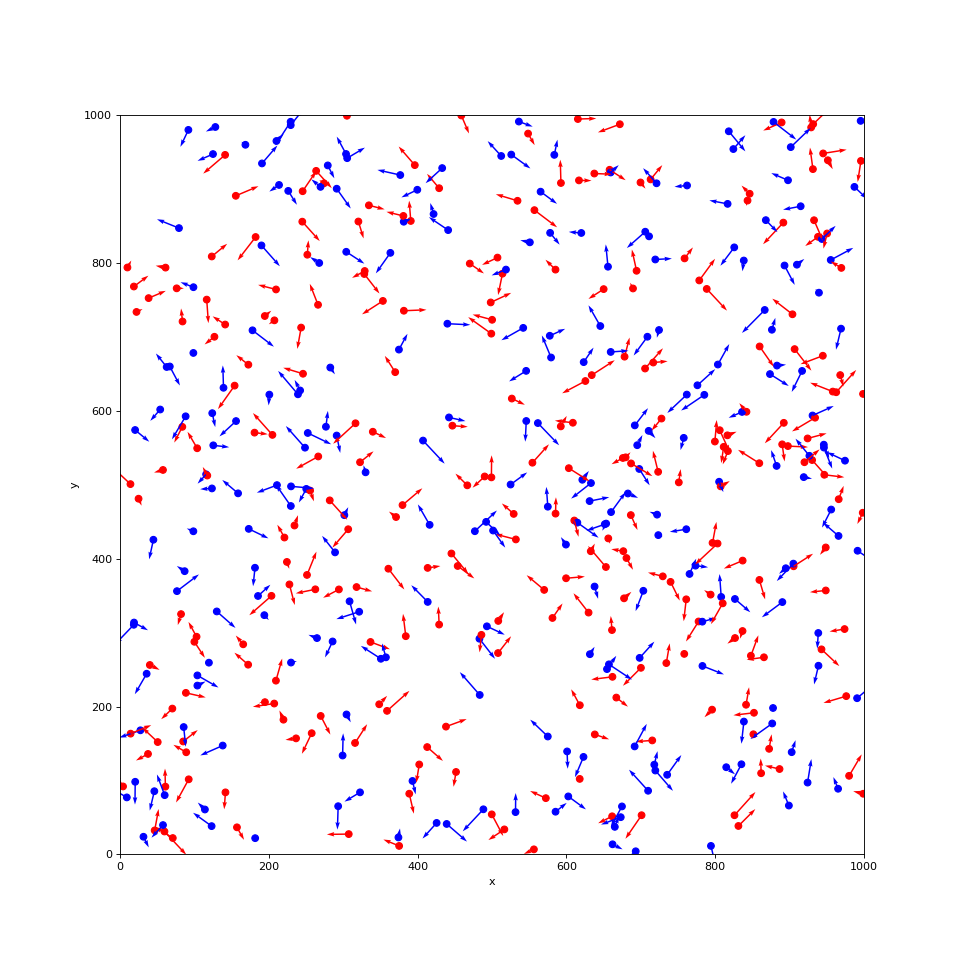
For our purposes, we really just want to be able to plot the positions of our boids and maybe some arrows to indicated their velocity.
~/code/vivarium_examples/boids/visualization.pydef plot_boids(simulation: InteractiveContext, plot_velocity: bool = False) -> None:
width = simulation.configuration.field.width
height = simulation.configuration.field.height
pop = simulation.get_population(["x", "y", "color", "vx", "vy"])
plt.figure(figsize=(12, 12))
plt.scatter(pop.x, pop.y, color=pop.color)
if plot_velocity:
plt.quiver(pop.x, pop.y, pop.vx, pop.vy, color=pop.color, width=0.002)
plt.xlabel("x")
plt.ylabel("y")
plt.axis((0, width, 0, height))
plt.show()
We can then visualize our flock with
from vivarium.engine import InteractiveContext
from vivarium_examples.boids.population import Population
from vivarium_examples.boids.movement import Movement
from vivarium_examples.boids.visualization import plot_boids

sim = InteractiveContext(
   components=[Population(), Movement()],
   configuration={'population': {'population_size': 500}},
   logging_verbosity=0,
)

plot_boids(sim, plot_velocity=True)
(Source code, png, hires.png, pdf)

Calculating neighbors
The steering behavior in the Boids model is dictated by interactions of each boid with its nearby neighbors. A naive implementation of this can be very expensive. Luckily, Python has a ton of great libraries that have solved most of the hard problems.
Here, we’ll pull in a KDTree from SciPy and use it to build a component that tells us about the neighbor relationships of each boid.
~/code/vivarium_examples/boids/neighbors.py 1from __future__ import annotations
2
3import pandas as pd
4from scipy import spatial
5
6from vivarium.engine import Component
7from vivarium.engine.framework.engine import Builder
8from vivarium.engine.framework.event import Event
9from vivarium.engine.framework.population import SimulantData
10
11
12class Neighbors(Component):
13 ##############
14 # Properties #
15 ##############
16 configuration_defaults = {"neighbors": {"radius": 60}}
17
18 #####################
19 # Lifecycle methods #
20 #####################
21
22 def setup(self, builder: Builder) -> None:
23 self.radius = builder.configuration.neighbors.radius
24
25 self.neighbors_calculated = False
26 self._neighbors = pd.Series()
27 builder.value.register_attribute_producer(
28 "neighbors", source=self.get_neighbors, required_resources=["x", "y"]
29 )
30 builder.population.register_initializer(
31 initializer=self.initialize_neighbors,
32 columns=None,
33 required_resources=[],
34 )
35
36 ########################
37 # Event-driven methods #
38 ########################
39
40 def initialize_neighbors(self, pop_data: SimulantData) -> None:
41 self._neighbors = pd.Series([[]] * len(pop_data.index), index=pop_data.index)
42
43 def on_time_step(self, event: Event) -> None:
44 self.neighbors_calculated = False
45
46 ##################################
47 # Pipeline sources and modifiers #
48 ##################################
49
50 def get_neighbors(self, index: pd.Index[int]) -> pd.Series[list[int]]: # type: ignore[type-var]
51 if not self.neighbors_calculated:
52 self._calculate_neighbors()
53 return self._neighbors[index]
54
55 ##################
56 # Helper methods #
57 ##################
58
59 def _calculate_neighbors(self) -> None:
60 # Reset our list of neighbors
61 pop = self.population_view.get(self._neighbors.index, ["x", "y"])
62 self._neighbors = pd.Series([[] for _ in range(len(pop))], index=pop.index)
63
64 tree = spatial.KDTree(pop[["x", "y"]])
65
66 # Iterate over each pair of simulants that are close together.
67 for boid_1, boid_2 in tree.query_pairs(self.radius):
68 # .iloc is used because query_pairs uses 0,1,... indexing instead of pandas.index
69 self._neighbors.iloc[boid_1].append(self._neighbors.index[boid_2])
70 self._neighbors.iloc[boid_2].append(self._neighbors.index[boid_1])
This component creates an attribute pipeline called neighbors so that other
components can access the neighbors of each boid (remember that every attribute
pipeline corresponds to a column in the population state table).
Note that the only thing it does in on_time_step is self.neighbors_calculated = False.
That’s because we only want to calculate the neighbors once per time step. When the pipeline
is called, we can tell with self.neighbors_calculated whether we need to calculate them
or use our cached value in self._neighbors.
Swarming behavior
Now we know which boids are each others’ neighbors but we’re not doing anything with that information. We need to teach the boids to swarm!
There are lots of potential swarming behaviors to play around with, all of which change the way that boids clump up and follow each other. But since that isn’t the focus of this tutorial, we’ll implement separation, cohesion, and alignment behavior identical to what’s in this D3 example (Internet Archive version), and we’ll gloss over most of the calculations.
We define a base class for all our forces, since they will have a lot in common.
We won’t get into the details of this class, but at a high level it uses the
neighbors attribute to find all the pairs of boids that are neighbors,
applies some force to (some of) those pairs, and limits that force to a maximum
magnitude.
~/code/vivarium_examples/boids/forces.pyclass Force(Component, ABC):
##############
# Properties #
##############
@property
def configuration_defaults(self) -> dict[str, dict[str, float]]:
return {
self.__class__.__name__.lower(): {
"max_force": 0.03,
},
}
#####################
# Lifecycle methods #
#####################
def setup(self, builder: Builder) -> None:
self.config = builder.configuration[self.__class__.__name__.lower()]
self.max_speed = builder.configuration.movement.max_speed
# docs-start: register_acceleration_modifier
    builder.value.register_attribute_modifier(
        "acceleration",
        modifier=self.apply_force,
        required_resources=["x", "y", "vx", "vy", "neighbors"],
    )
# docs-end: register_acceleration_modifier
##################################
# Pipeline sources and modifiers #
##################################
def apply_force(self, index: pd.Index[int], acceleration: pd.DataFrame) -> pd.DataFrame:
neighbors = self.population_view.get(index, "neighbors")
pop = self.population_view.get(index, ["x", "y", "vx", "vy"])
if not (isinstance(neighbors, pd.Series) and isinstance(pop, pd.DataFrame)):
raise ValueError(
"Neighbors must be a pd.Series of ints and population a pd.DataFrame"
)
pairs = self._get_pairs(neighbors, pop)
raw_force = self.calculate_force(pairs)
force = self._normalize_and_limit_force(
force=raw_force,
velocity=pop[["vx", "vy"]],
max_force=self.config.max_force,
max_speed=self.max_speed,
)
acceleration.loc[force.index, "acc_x"] += force["x"]
acceleration.loc[force.index, "acc_y"] += force["y"]
return acceleration
##################
# Helper methods #
##################
@abstractmethod
def calculate_force(self, neighbors: pd.DataFrame) -> pd.DataFrame:
pass
def _get_pairs(
self, neighbors: pd.Series[int | float], pop: pd.DataFrame
) -> pd.DataFrame:
pairs = (
pop.join(neighbors.rename("neighbors"))
.reset_index()
.explode("neighbors")
.merge(
pop.reset_index(),
left_on="neighbors",
right_index=True,
suffixes=("_self", "_other"),
)
)
pairs["distance_x"] = pairs.x_other - pairs.x_self
pairs["distance_y"] = pairs.y_other - pairs.y_self
pairs["distance"] = np.sqrt(pairs.distance_x**2 + pairs.distance_y**2)
return pairs
def _normalize_and_limit_force(
self,
force: pd.DataFrame,
velocity: pd.DataFrame,
max_force: float,
max_speed: float,
) -> pd.DataFrame:
normalization_factor = np.where(
(force.x != 0) | (force.y != 0),
max_speed / self._magnitude(force),
1.0,
)
force["x"] *= normalization_factor
force["y"] *= normalization_factor
force["x"] -= velocity.loc[force.index, "vx"]
force["y"] -= velocity.loc[force.index, "vy"]
magnitude = self._magnitude(force)
limit_scaling_factor = np.where(
magnitude > max_force,
max_force / magnitude,
1.0,
)
force["x"] *= limit_scaling_factor
force["y"] *= limit_scaling_factor
return force[["x", "y"]]
def _magnitude(self, df: pd.DataFrame) -> pd.Series[float]:
return pd.Series(np.sqrt(np.square(df.x) + np.square(df.y)), dtype=float)
The major new Vivarium feature seen here is that of the attribute modifier,
which we register with vivarium.engine.framework.values.interface.ValuesInterface.register_attribute_modifier().
As the name suggests, this allows us to modify attributes,
in this case adding the effect of a force to the acceleration attribute.
We register that the apply_force method as the modifier like so:
~/code/vivarium_examples/boids/forces.py builder.value.register_attribute_modifier(
"acceleration",
modifier=self.apply_force,
required_resources=["x", "y", "vx", "vy", "neighbors"],
)
Once we start adding components with these modifiers into our simulation, acceleration won’t always be zero anymore!
We then define our three forces using the Force base class.
We won’t step through what these mean in detail.
They mostly only override the _calculate_force method that calculates the force between a pair
of boids.
The separation force is a bit special in that it also defines an extra configurable
parameter: the distance within which it should act.
~/code/vivarium_examples/boids/forces.pyclass Separation(Force):
"""Push boids apart when they get too close."""
configuration_defaults = {
"separation": {
"distance": 30,
"max_force": 0.03,
},
}
def calculate_force(self, neighbors: pd.DataFrame) -> pd.DataFrame:
# Push boids apart when they get too close
separation_neighbors = neighbors[neighbors.distance < self.config.distance].copy()
force_scaling_factor = np.where(
separation_neighbors.distance > 0,
((-1 / separation_neighbors.distance) / separation_neighbors.distance),
1.0,
)
separation_neighbors["force_x"] = (
separation_neighbors["distance_x"] * force_scaling_factor
)
separation_neighbors["force_y"] = (
separation_neighbors["distance_y"] * force_scaling_factor
)
force: pd.DataFrame = (
separation_neighbors.groupby("index_self")[["force_x", "force_y"]]
.sum()
.rename(columns=lambda c: c.replace("force_", ""))
)
return force
class Cohesion(Force):
"""Push boids together."""
def calculate_force(self, pairs: pd.DataFrame) -> pd.DataFrame:
return (
pairs.groupby("index_self")[["distance_x", "distance_y"]]
.sum()
.rename(columns=lambda c: c.replace("distance_", ""))
)
class Alignment(Force):
"""Push boids toward where others are going."""
def calculate_force(self, pairs: pd.DataFrame) -> pd.DataFrame:
return (
pairs.groupby("index_self")[["vx_other", "vy_other"]]
.sum()
.rename(columns=lambda c: c.replace("v", "").replace("_other", ""))
)
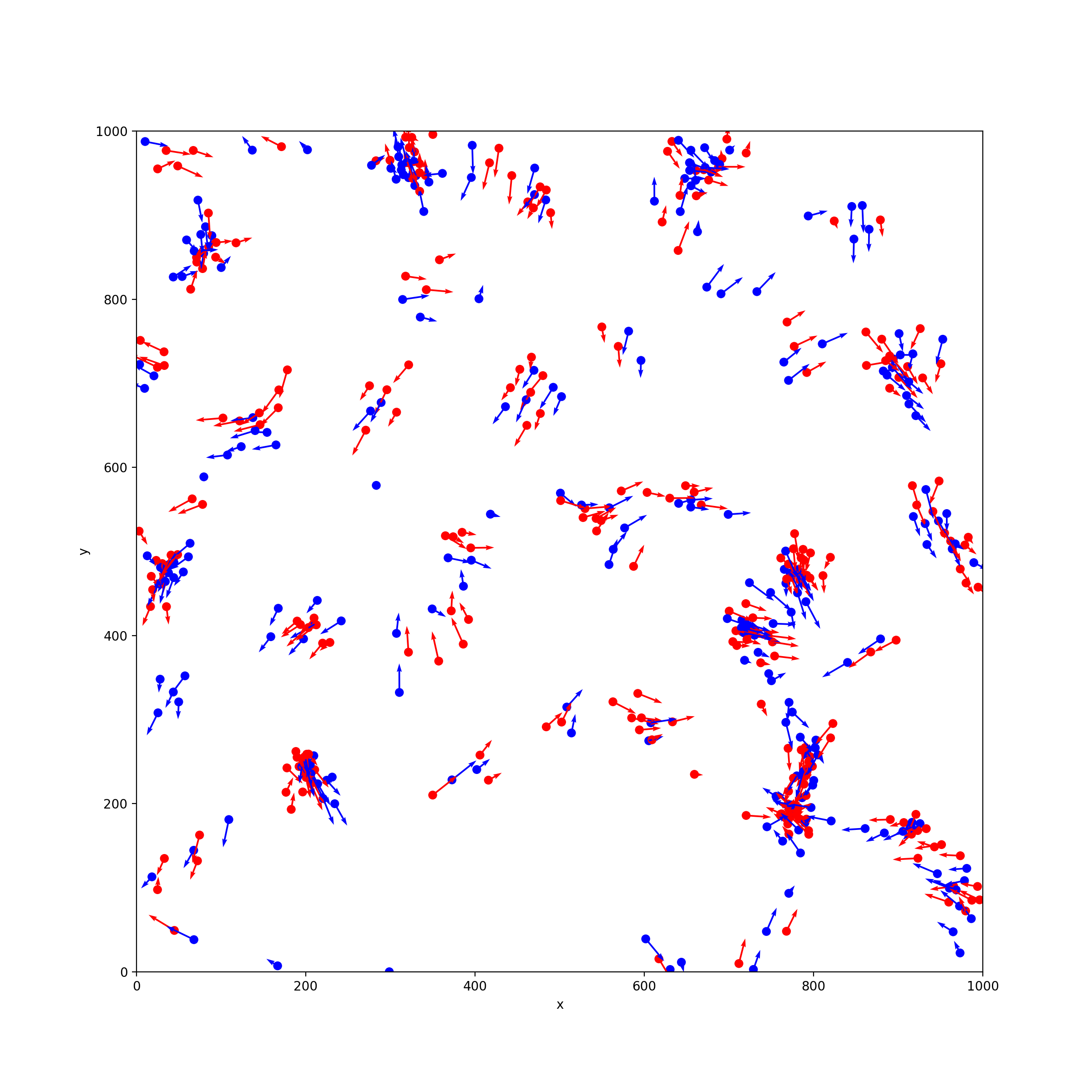
For a quick test of our swarming behavior, let’s add in these forces and check in on our boids after 100 steps:
from vivarium.engine import InteractiveContext
from vivarium_examples.boids.population import Population
from vivarium_examples.boids.movement import Movement
from vivarium_examples.boids.neighbors import Neighbors
from vivarium_examples.boids.forces import Separation, Cohesion, Alignment
from vivarium_examples.boids.visualization import plot_boids

sim = InteractiveContext(
   components=[Population(), Movement(), Neighbors(), Separation(), Cohesion(), Alignment()],
   configuration={'population': {'population_size': 500}},
   logging_verbosity=0,
)

sim.take_steps(100)

plot_boids(sim, plot_velocity=True)
(Source code, png, hires.png, pdf)

Viewing our simulation as an animation
Great, our simulation is working! But it would be nice to see our boids moving around instead of having static snapshots. We’ll use the animation features in matplotlib to do this.
Add this method to visualization.py:
~/code/vivarium_examples/boids/visualization.pydef plot_boids_animated(simulation: InteractiveContext) -> FuncAnimation:
width = simulation.configuration.field.width
height = simulation.configuration.field.height
pop = simulation.get_population(["x", "y", "color"])
fig = plt.figure(figsize=(12, 12))
ax = fig.add_subplot(111)
s = ax.scatter(pop.x, pop.y, color=pop.color)
plt.xlabel("x")
plt.ylabel("y")
plt.axis((0, width, 0, height))
frames = range(2_000)
frame_pops = []
for _ in frames:
simulation.step()
frame_pops.append(simulation.get_population(["x", "y"]))
def animate(i: int) -> None:
s.set_offsets(frame_pops[i])
return FuncAnimation(fig, animate, frames=frames, interval=10) # type: ignore[arg-type]
Then, try it out like so:
from vivarium.engine import InteractiveContext
from vivarium_examples.boids.population import Population
from vivarium_examples.boids.movement import Movement
from vivarium_examples.boids.neighbors import Neighbors
from vivarium_examples.boids.forces import Separation, Cohesion, Alignment
from vivarium_examples.boids.visualization import plot_boids_animated

sim = InteractiveContext(
    components=[Population(), Movement(), Neighbors(), Separation(), Cohesion(), Alignment()],
    configuration={'population': {'population_size': 500}},
    logging_verbosity=0,
 )

anim = plot_boids_animated(sim)
Viewing this animation will depend a bit on what software you have installed. If you’re running Python in the terminal, this will save a video file:
anim.save('boids.mp4')
In IPython, this will display the animation:
HTML(anim.to_html5_video())
Either way, it will look like this: